Soil Property Prediction from Public Spectral Data

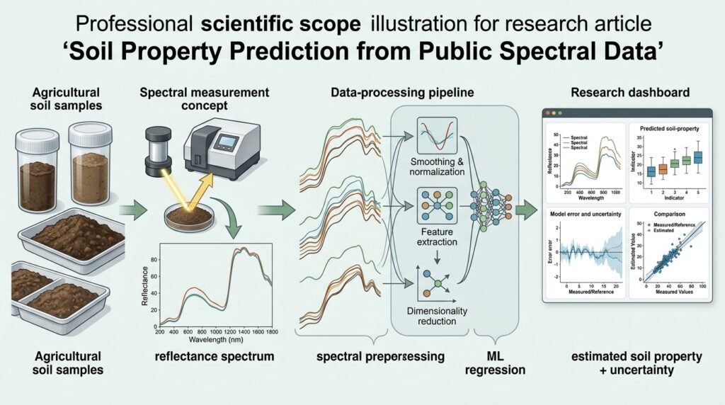
A research project that estimates measurable soil properties — organic carbon, pH, texture fractions — from diffuse-reflectance spectra using the European Union’s LUCAS topsoil spectral library. The workflow is chemometrics: preprocess the reflectance spectra, transform wavelength features, train regression models, and report per-property errors with uncertainty — always against laboratory reference values, which remain the ground truth this kind of model can approximate but never replace. It is the site’s most research-oriented machine-learning Idea: a rigorous, notebook-first project for people who want their regression skills tested by a genuinely hard, genuinely useful scientific problem.

>Estimation, not prescription. The model estimates selected soil properties from spectral measurements. It does not recommend fertilizers, chemical amendments, or treatment dosages, and it makes no claims of guaranteed soil improvement. Laboratory analysis remains the reference method; spectral prediction is a fast, cheap screening complement whose errors must be understood before anyone acts on a single number it produces.

Who Is This For?

• Soil scientists who want a reproducible spectral-prediction baseline they can extend and cite
• Precision-agriculture researchers evaluating whether spectral screening fits their workflows
• Agri-data students ready for an advanced regression project with real scientific texture
• Chemometrics learners who want the classical preprocessing-and-validation discipline applied to modern ML

The Problem

Conventional soil analysis is slow and expensive: samples are collected in the field, shipped to laboratories, and processed with wet-chemistry methods that can take weeks per batch. Soil sensing by diffuse reflectance spectroscopy offers a fast, comparatively cheap alternative — shine light across a wavelength range, record how the soil reflects it, and infer properties from the spectral signature. The approach is established in the research literature, and the EU’s Land Use/Cover Area frame Survey (LUCAS) has published one of the world’s largest harmonized collections of topsoil samples with both laboratory-measured properties and corresponding spectra. What’s missing for most learners is a walkable path through it: how to preprocess spectra defensibly, how to avoid the validation traps that inflate published accuracies, and how to report uncertainty so results mean something to a soil scientist. The gap between “there is a giant public spectral library” and “I have a validated, honestly-reported prediction model” is this project.

How It Works

Spectral regression is chemometrics — a century-old discipline with hard-won rules about preprocessing and validation. The pipeline below follows those rules while using modern ML tools.

1. Obtain and Inspect the Spectral Library

Download a LUCAS topsoil data package from the European Soil Data Centre (free after registration), which pairs soil property measurements (organic carbon, pH, particle-size fractions, and others) with the corresponding reflectance spectra. Inspect before modeling: wavelength range and resolution, sample counts, property distributions, geographic coverage of the sampling sites, and — critically — the documented measurement protocols. Provenance is part of the science: record which data package version you used and when.

2. Inspect Data Quality

Spectral datasets carry real-world noise: anomalous spectra (sensor glitches, moisture artifacts), samples with missing or censored property values, and sites measured under different conditions. Build a quality-inspection step that flags spectra with implausible reflectance values, reports missing-value patterns per property, and visualizes a random sample of spectra so you can see what typical and atypical look like. Decide and document exclusion rules before you look at any model results — otherwise quality filtering quietly becomes accuracy tuning.

3. Preprocess the Spectra

Raw reflectance carries scattering and baseline effects that swamp the chemical signal. Classical chemometric preprocessing exists precisely for this: continuum removal or standard normal variate (SNV) transforms to separate absorption features from scattering baselines; Savitzky–Golay smoothing and its derivative filters to sharpen absorption features; and band selection or resampling to reduce redundancy. Apply preprocessing fitted on training data only where any parameters are learned, and treat the preprocessing choice itself as an experiment — different transforms measurably change which properties are predictable.

4. Split with Geography in Mind

Random sample-level splits overstate performance when nearby sampling sites share geology, climate, and parent material. The honest default is a spatially aware evaluation: at minimum, group samples by region so that spatially clustered neighbors do not straddle train and test; ideally, hold out entire regions. Report both a random split and a spatial split — the gap between the two numbers is itself a scientific finding about geographic generalization.

5. Train Regression Models

For each target property, train regression models on the preprocessed spectra. Classical chemometrics starts with partial least squares regression (PLSR) — the domain’s workhorse, interpretable and strong on collinear spectra. Compare it against modern baselines: ridge regression on transformed features, random forests, gradient boosting, and optionally a small neural network. Keep the per-property discipline: organic carbon, pH, and clay behave very differently spectrally, and a single pooled model hides that. Dimensionality reduction (PCA) and feature selection across wavelengths are legitimate experiments here — spectra are highly collinear, and the wavelength-region importance you recover is interpretable science (clay minerals, organic matter, and iron oxides all have known absorption features).

6. Evaluate with Error and Uncertainty

Report per-property error metrics (RMSE, MAE, bias, and the ratio of performance to deviation common in soil-science literature) on the held-out split — never on resubstitution of training samples. Add uncertainty: prediction intervals via bootstrapped models or quantile regression, and residual analysis against properties not modeled (does organic-carbon error grow on sandy samples?). Publish the errors next to the analytical precision of the laboratory reference method itself, because “close to the lab” is the meaningful yardstick, and the lab is not perfect either.

7. Interpret and Document

The research deliverable is not just a model but an understanding: which wavelength regions drove predictions, which properties were predictable and which were not, how spatially portable the model is, and where it fails. Document preprocessing parameters, package versions, and split definitions so another researcher can reproduce the study exactly. This is the part that turns a good project into a citable one.

Key Features

• Spectral regression pipeline for multiple soil properties with per-property models
• Classical chemometric preprocessing — SNV/continuum removal, Savitzky–Golay smoothing and derivatives
• Spatially aware validation — region-grouped and region-held-out splits alongside random splits
• Uncertainty reporting — prediction intervals and residual analysis, not just point estimates
• Model comparison — PLSR against modern ML baselines with identical validation
• Full provenance — dataset version, preprocessing parameters, and split definitions recorded for reproducibility

Functional Requirements

• Load a LUCAS topsoil package: spectra plus paired laboratory-measured properties
• Quality-inspect spectra and property values with documented, pre-registered exclusion rules
• Apply configurable preprocessing chains (SNV, continuum removal, smoothing, derivatives) fitted on training data only
• Train per-property regression models (PLSR baseline plus at least two ML baselines)
• Evaluate with region-aware splits, per-property error metrics, and prediction intervals
• Export a research report: per-property results, preprocessing comparison, failure analysis, and complete reproducibility notes

User Stories

• As a soil scientist, I want per-property errors with uncertainty so I can judge whether spectral screening fits my program.
• As a researcher, I want region-held-out results so I know how the model travels beyond sampled geography.
• As a student, I want the preprocessing experiments scripted so I can see what each transform does to the spectra and the errors.
• As a reviewer, I want split definitions and package versions recorded so I can reproduce the study.
• As a data scientist, I want PLSR as a baseline so I can tell whether fancy models actually beat the classical method.

MVP Scope

A minimal but complete MVP:

Explicitly out of MVP: multi-property joint models, transfer across instruments, field-moisture corrections, and mapping predictions spatially. All are natural extensions.

Project Timeline

• Week 1: data acquisition, inspection, quality rules, preprocessing experiments
• Week 2: PLSR baseline, validation design, first honest results
• Week 3: ML baselines, spatial-split comparison, uncertainty estimation
• Week 4: failure analysis, research report, reproducibility package, polish

Testing Strategy

• Validation tests: no sample’s region straddles train and test in grouped splits; preprocessing parameters fitted on training folds only
• Reproducibility tests: the full pipeline reruns from a clean checkout to the same numbers under a fixed seed
• Sanity tests: predictions on spectra held out from known-property samples fall within plausible physical ranges; per-property errors worse than naive climatology (predicting the training mean) is treated as a bug, not a result
• Data tests: every spectrum pairs with a valid property value or is excluded per the documented rules; exclusion counts reported

Success Metrics

• Measured per-property RMSE, MAE, and bias for every modeled property on a region-grouped held-out split (your own numbers)
• A random-split vs spatial-split comparison reported, with the generalization gap discussed rather than hidden
• Prediction intervals or bootstrapped uncertainty accompanying every point estimate
• The full study reruns from a clean checkout to identical numbers, with preprocessing parameters and split definitions recorded
• A failure analysis identifying which samples and conditions the model handles worst, and why

Common Challenges

• Preprocessing whack-a-mole — trying transforms until test metrics look good is silent overfitting; fix the evaluation design first, then compare preprocessing as a reported experiment
• Collinearity everywhere — adjacent wavelengths are highly correlated; models that look impressive on training data may be memorizing smoothness rather than chemistry
• Spatial autocorrelation — nearby sites share parent material and climate; random splits leak geography, which is why grouped splits are the default here
• Property-specific behavior — spectrally active properties (organic carbon) predict far better than weakly expressed ones; a single headline number across properties misleads
• Reference-method limits — the lab values carry their own error; chasing model RMSE below the reference method’s analytical variability is chasing noise

Learning Objectives

• Apply classical chemometric preprocessing (SNV, continuum removal, Savitzky–Golay derivatives) and understand what each corrects
• Design spatially honest validation for geographically clustered data
• Build and compare regression models — PLSR against modern ML baselines — under identical, leakage-free evaluation
• Report uncertainty alongside point estimates and relate model error to reference-method precision
• Document a research study to reproducibility standards: provenance, parameters, splits, and versions

Research Ethics and Data Considerations

• Retain provenance end to end. Record the dataset version, download date, exclusion rules, preprocessing parameters, and split definitions with the results — a spectral model without provenance is not reproducible research.
• Respect the ESDAC/LUCAS access terms: the data is free after registration; do not redistribute the raw package in ways the license forbids, and cite the dataset and its documentation in anything derived from it.
• Laboratory reference values carry their own uncertainty. Report model errors alongside the documented analytical variability of the reference methods; presenting model output as more authoritative than the lab is exactly backwards.
• Scope the claims: a model trained on one survey’s sampling distribution says nothing definitive about soils, instruments, or regions it never saw. State the coverage; resist the temptation to generalize.

Limitations

• Preprocessing sensitivity — results can swing materially with the transform choice; report preprocessing experiments rather than a single configuration
• Reference-method uncertainty — lab values themselves carry error; the model cannot be more accurate than its ground truth allows
• Geographic domain shift — soil-forming factors differ across regions; performance decays outside the sampled distribution, and spatial splits quantify exactly that
• Instrument and condition effects — moisture, measurement geometry, and sensor differences alter spectra; cross-instrument transfer is a research problem of its own
• Property coverage — some properties are spectrally active (organic carbon, iron oxides) and predictable; others are weakly expressed and harder; per-property honesty is mandatory
• No prescription — outputs are property estimates for research and screening; they never translate into fertilizer or amendment recommendations

Why This Idea Is Different

The site’s agricultural Ideas answer different questions with different data. The AI Crop Yield Estimator from Field & Weather Data forecasts how much a field will produce from field, soil, and weather history — a forecasting task on environmental time series. The GMO Trait Analysis Explorer for Agricultural Researchers explores curated trait and identifier records — a data-exploration tool over structured biological annotations. This project predicts laboratory-measurable soil properties from spectral signatures — chemometric regression where the features are wavelengths and the ground truth is wet-chemistry analysis. Different inputs (spectra, not weather or trait tables), different model class (calibrated regression against lab references, not forecasting or record browsing), and a research audience of soil scientists rather than farm planners. All three share the agriculture domain and the honesty-about-uncertainty discipline, which is precisely why they cross-link as a family.

What Similar Tools Exist

| Tool type | Approach | Limitation |
|———–|———-|————|
| Commercial soil-spectral services | Vendor models with proprietary calibrations | Opaque; errors and coverage undisclosed; costly per sample |
| Research lab pipelines | In-house chemometrics | Not reproducible outside the lab; rarely documented for learners |
| Generic regression tutorials | Standard ML on toy datasets | No spectral physics, no chemometric discipline, no reference-method context |
| Lab analysis alone | Wet chemistry per sample | Slow and expensive at survey scale; the reference, not the screener |

This project’s differentiators: a fully reproducible pipeline on the largest harmonized public soil spectral library, classical-to-modern model comparison under identical validation, spatially honest evaluation, uncertainty reporting, and an explicit no-prescription boundary.

Technology Stack

• Python — the whole pipeline
• pandas / NumPy — data handling and spectral matrices
• scikit-learn — PLSR, ridge, forests, boosting, cross-validation utilities
• scipy / savgol filtering — Savitzky–Golay smoothing and derivatives
• matplotlib — spectra, residuals, and per-property diagnostics
• Jupyter notebooks — the research narrative and reproducibility package

Future Enhancements

• Cross-instrument transfer experiments (library-to-field spectrometer)
• Multi-task models predicting several properties jointly with shared representations
• Soil-grid mapping: combine predictions with spatial covariates for regional maps
• Moisture-effect studies: how wet-sample spectra distort predictions and how to correct
• Open benchmarking: publish the split definitions so others can compare models fairly

Related Ideas

• AI Crop Yield Estimator from Field & Weather Data — agricultural forecasting on environmental time series vs this project’s spectral regression
• GMO Trait Analysis Explorer for Agricultural Researchers — structured trait-data exploration vs this project’s laboratory-reference modeling
• Automated Data Quality Scorecard for Data Teams — the data-quality discipline this project applies to spectral libraries

Browse more Research Ideas · Advanced Ideas